|
 |
Is there any data to support the Six Sigma's plus or minus 1.5 sigma shift?
[ Posted by: Lynn Rhodes ]
|
I worked for Motorola, Inc. from 1984 to 1991. My direct responsibility, as head of the department of statistical methods, was to implement and disseminate the use of statistical methods to achieve and sustain Motorola's corporate quality "Five Year Goal" which was: "Achieve Six Sigma Capability by 1992 - in Everything We Do".
When the document "Our Six Sigma Challenge" was distributed on January 15, 1987, it made reference to the plus or minus 1.5-sigma shift, and to the 3.4-ppm defect level. When I sought more factual details to support these statements, the facts were always "anecdotal". There was no data, no hard analysis, no conclusive evidence, and no statistical validation to these assertions.
As the inquiries grew, so did the doubt about the quality goal. Later in 1988, Mikel Harry and Riegle Stewart came to the rescue to add credibility to the statements by publishing an internal document "Six Sigma Mechanical Design Tolerancing". This document again presented no data to support any validation of the 1.5 sigma shift, however, it makes reference to articles written by David H. Evans and A. Bender.
If you follow the trail by reading the articles:
- David H. Evans, "Statistical Tolerancing: The State of the Art, Part I. Background," Journal of Quality Technology, Vol. 6 No.4, (October 1975), pp. 188-195,
- David H. Evans, "Statistical Tolerancing: The State of the Art, Part I. Methods for Estimating Moments," Journal of Quality Technology, Vol. 7 No.1, (January 1975), pp. 1-12,
- David H. Evans, "Statistical Tolerancing: The State of the Art, Part II. Shifts and Drifts," Journal of Quality Technology, Vol. 7 No.2, (April 1975), pp. 72-76, and
- A. Bender, "Benderizing Tolerances - A Simple Practical Probability Method of Handling Tolerances for Limit-Stack-Ups, "Graphic Science, (December 1962), pp. 17-21,
you will probably find, as I did, that there is nothing to substantiate the plus or minus 1.5 sigma shift.
I can assert that there was never any data to support the "plus or minus 1.5 sigma shift".
Anyone can make claims about the 1.5 sigma shift, but I was there -inside Motorola- and can firmly say that there was never any data to support the 1.5 sigma shift. In 1987, Bob Galvin did not have it, Jack Germain did not have it, Bill Smith did not have it, Mikel Harry did not have it, Riegle Stewart did not have it, and I could not get it either.
It is a known fact that processes vary. By how much, we do not know. The second law of thermodynamics tells us that left to itself, the entropy (or disorganization) of any system can never decrease. Although we cannot completely defeat this law, we can appease it by forcing the system (a process) to a state of functional equilibrium by process monitoring and process adjustments, hence, statistical process control.
My suggestion is to put this illegitimate subject to rest and instead focus on something more meaningful, such as using Six Sigma approach to optimize processes.
by MARIO PEREZ-WILSON
|
|
|
I have been coordinating Six Sigma in a global organization and have seen many incorrect applications of DOEs. How can you avoid these mistakes?
[ Posted by: Anthony ]
|
|
I cannot deny that I have seen my share of inappropriate applications of design of experiments in my professional career.
One of the challenges of implementing Six Sigma, MPCpS, TQM or any improvement initiative in large organizations is that when the momentum increases rapidly, you will find that many teams will be at a point of improving or optimizing their processes at once. The stage of improvement or optimization is the stage where the processes get fixed. This is the stage with the longest cycle time since it requires finding a solution to the root-cause of the problem, and this involves planning, designing, conducting and analyzing experiments.
If you are not well prepared to provide the proper guidance or coaching when many teams and individuals are ready to design and run experiments, you may experience a high level of misapplications.
Many times team members believe they have enough knowledge to plan, design and conduct their own experiments and they may not seek guidance a priori to save time. However, once they find out that their DOE does not bring the expected results, or the error term is so large that nothing appears to be significant, they may seek help from the statistician.
Nothing seems to be more annoying than hearing the words, "Can you analyze this data from an experiment we ran?" particularly when the statistician was never involved in the design of the experiment.
If an experiment has flaws in the design or in its execution, there isn't a sophisticated analytical tool that may extract useful and conclusive information from the experimental data. The design has to be flawless and its execution often requires controlled supervision by a statistician, particularly to apply a contingent plan to salvage the design in case of an accidental miscarriage.
During the deployment of Six Sigma at Motorola, I implemented a very simple and useful remedy to ascertain that experiments were designed properly prior to being conducted. The remedy was named Request for Engineering Experiment, REEX.
REEX is a form that requires answers to questions about the problem being solved, the design of the experiment, its execution, disposition of the product and appropriate approval. At the pinnacle of the Six Sigma deployment at Motorola, we were running hundreds of experiments a week.
Experiments require the allocation of product, material, equipment, gauges, machines, and processes, as well as production, engineering, and maintenance personnel, not to mention the alteration of scheduled downtime, which amounts to significant cost expenses. For this reason, experiments need to be managed and controlled to guarantee success and efficiency.
The typical subjects included in the REEX are:
- Purpose of the experiment
- Type of problem being solved
- List of independent variables
- List of responses and its µ, sigma, GR&R,
- Expected response curve
- Test vehicle
- Alpha error, randomization, replication
- Model
- Cost, etc.
|
|
|
In Design of Experiments they refer to factors being nested or crossed. How can you tell the difference?
[ Posted by: Jeff Brooks ]
|
"Nested" or "crossed" refers to the relationship between factors.
Imagine that you are running an experiment with four factors: Vineyard, Grape-Type (or Must), Temperature of Fermentation, and Filtering, and that you are measuring a particular response.
For the factor Vineyard, you have chosen to compare two vineyards one in France and one in Chile.
For Grape-Type, imagine that both vineyards have Chardonnay and Sauvignon Blanc grapes planted from the same root vine, and the same amount of must is harvested and used in the experiment.
For Temperature of Fermentation you select two levels, 10 degrees Centigrade and 30 degrees Centigrade. (Let's assume the temperature can be controlled very accurately).
Finally, for Filtration, you have selected two filter types, one from a company call Pall-Bio and the other from Kieselguhr, and both types of filters are shipped to the vineyards.
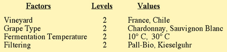
Fig 1. Factors, Levels and Values in a Nested Experiment
Let's examine the relationship between the factors in this experiment.
The relationship between Vineyard and Grape-Type is NESTED.
In this example, it should be obvious that the factor "Grape-Type" is nested or uniquely contained within the levels of Vineyard. At each level of Vineyard, we have Chardonnay and Sauvignon Blanc. The Chardonnay in France, will be different than the Chardonnay in Chile, and the Sauvignon Blanc in Chile, will be different from the one in France. Even though they came from the same original root vine, they will be different due to other influential conditions. The name of the levels may be the same, but the grapes (Chardonnay and Sauvignon Blanc) are different at each level of the factor Vineyard. So, the factor Grape-Type is nested within the factor Vineyard. Nested, as the word implies, means contained within.
The relationship between Grape-Type and Fermentation Temperature is CROSSED.
Here, both Chardonnay and Sauvignon Blanc will be fermented at two distinct temperatures, 10 and 30 degrees Centigrade. 10 degrees Centigrade, will be the same in France as it is in Chile. The same goes for 30 degrees Centigrade. So here the relationship between Grape-Type and Fermentation Temperature is that these two factors are crossed. In other words, the levels of Temperature of Fermentation are the same at each level of Grape-Type.
The relationship between Fermentation Temperature and Filtering is CROSSED.
Again, the filtering is done at two levels using the filters from Pall-Bio and the filters from Kieselguhr. Both filters were shipped to each Vineyard, so these two levels are the same. So, in this case, Temperature and Filtering are also crossed factors.
Now, let's say that we decided to replicate the experiment. Replication is always nested.
I have drawn a Tier-Relation Diagram that may help you visualize the relationship between crossed and nested factors in the experiment.
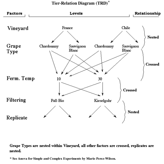
Fig 2. Tier-Relation Diagram for DOE Experiment
Hope this is helpful.
by MARIO PEREZ-WILSON
|
|
|
What was the episode that made Motorola to develop Six Sigma? Some of the authors I've read said that in the 70s one Japanese company acquired one TV factory from Motorola. This Japanese company done a complete change in the management, and soon the factory was producing TV sets with only 5% the number of defects they had produced under Motorola management. Do you agree with this affirmation?
[ Posted by: Eliane ]
|
This story about the TV set is nonsense. Something that happened in the 1970s did not trigger a reaction 16 years later. Motorola under Bob Galvin was very fast in reacting. See below the Motorola Sector Imperatives, in particular, the enabling imperative: Speed of Execution.
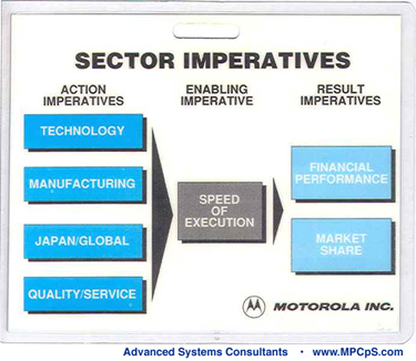
Fig 1. Enabling Imperative: Speed of Execution.
The episode which triggered six sigma (the quality goal) was the development of total customer satisfaction as a business strategy to increase business:
Timeframe: Jul-1986 Jan-1987
In the third and fourth quarter of 1986, Bob Galvin, CEO of Motorola, visited a number of key customers.
Some of the customers complained that they were not being served well. There were on-time delivery issues, issues related to accuracy in transactions, wrong parts were shipped with orders, orders not completed properly, and also quality issues. So Bob asked these individuals who complained. If we fixed these problems from now on, how much business (orders) would they give Motorola?
Bob Galvin came back to Motorola at the end of his customer visits, and announced to his employees that our customers have agree to give us 5% to 20% more business if we could served then from a total quality standpoint.

Fig 2. Total Customer Satisfaction - Motorola's Fundamental Objective.
Bob further develops the total quality statement with a revision to the Corporate Quality Goal. The "Revised Corporate Quality Goal", which was issued on Jan 15 1987, included the following:
- Improve products and services 10 times by 1989
- One hundred fold by 1991
- Achieve Six Sigma Capability by 1992.
Six Sigma (Process) Capability means having a Process Potential (Cp) of 2, and Process Capability Index (Cpk) of 2.
- Zero defects
- Total Customer Satisfaction (TCS).
So, the revised quality goal triggers Motorola's strategic objective "Our Fundamental Objective" of "Total Customer Satisfaction."
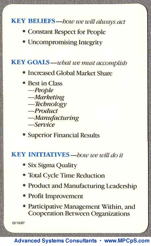
Fig 3. Motorola's Key Beliefs, Key Goals, and Key Initiatives.
The strategic objective of TCS has three elements: Key Beliefs, Key Goals, Key Initiatives.
One of the Key Initiatives is Six Sigma Quality. At this point in time (1987) Six Sigma was a quality goal of process capability, which gives ZERO defects.
A methodology or a blueprint, which the employees could follow to achieve Six Sigma was non-existent as that point in time. Six Sigma was just a quality goal, and what trigged it was a brilliant business strategy.
Hope this helps.
by MARIO PEREZ-WILSON
|
|
|
Is there a way to guardband the tolerance once I know the Gauge R&R?
[ Posted by: Eileen ]
|
|
Off course tolerances and specification limits can be guard banded once you know the gauge standard deviation.
Guard Banding Specification Limits
Consider an interest in guard banding the specification limits to tightened limits.
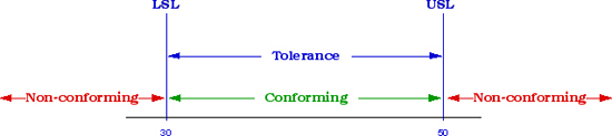
Fig 1. Tolerances and Specification Limits for Guard Banding
Let us assume, the product has a LSL=30, USL=50 and the gauge standard deviation is s=1.01.
We can compute a median uncertainty for a measurement, estimated at ±0.67s, which would bracket 50% of the uncertainties (assuming a normal distribution).
This can be done for both sides of the specification limits.
The median uncertainty would be ±0.67, and would give a Tightened Guard Band at the lower specification limit equal to 30.67 and a 49.33 for the upper specification limit.
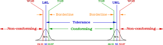
Fig 2. Guard Banded Tolerances and Specification Limits
TGB - Tightened Guard Band
WGB - Widened Guard Band
During production inspection or testing, all units within the tightened guard band specification limits (TGB) are likely to be conforming. All units which fall in between the guard band limits (within WGB and TGB) are considered to be borderline and should be dispositioned based on retesting. All units beyond the widened guard band limits are highly likely to be non-conforming.
To contain approximately 95% of the uncertainties, we can use a more conservative guard band set at ±2s.
Hope this helps.
by MARIO PEREZ-WILSON
|
|
|
What is the appropriate sample size to calculate the Cpk?
[ Posted by: Janice Johnson ]
|
The Cpk formula has two values that vary from sample to sample. These are the mean and the sigma, where the sigma is estimated by the sample standard deviation. The mean also varies, but to a larger degree the sigma may be a more important statistic.
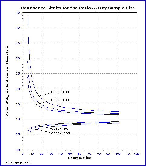
Fig 1. Confidence Limits for the Ratio of Sigma to Standard Deviation
In the Y-Axis, we have sigma (the parameter or population standard deviation) divided by the sample standard deviation. When they are equal, we have 1.0. The graph shows a horizontal line at 1.0.
In the graph, we can see that the confidence limits converge to 1.0 as the sample size increases. This implies that as the sample sizes become larger, the sample standard deviations are better estimates of the sigma (population standard
deviation).
For example, let's examine the implications to the standard deviation when we take a sample size of 31 observations (30 degrees of freedom, df) compared to a sample size of 101 observations (100 df).
Using a confidence limit (CL) at 5% and n=31, from the graph we get 0.785, and at CL=95% and n=31, we get 1.208. This implies that 90 percent of the time, sigma (the parameter being estimated) will be contained by this interval [0.785-1.208]. Let's say you have a characteristic measured in inches and the value of the sample standard deviation was 2.85 inches, then the confidence interval 2.24 (2.85 x 0.785) and 3.44 (2.85 x 1.208) will contain the sigma of the characteristic. In other words, at the 90 percent confidence level, the standard deviation is good to within -21.5% and +20.8%.
Now, at CL=5% and n=101, from the graph we get 0.883, and at CL=95% and n=101, we get 1.115. With a sample size of 101, and with a 90 percent degree of confidence, the standard deviation is good to within -11.7% and +11.5%. By increasing the sample size, the length of the confidence interval is much shorter; it went from 42.3 to 23.2. That is a 45.15% reduction.
What are the implications to the Cpk? The larger the sample size the shorter the confidence interval, and the better my prediction.
In short, when it's economically feasible, you should try to increase the sample size to at least 100 observations. 200 would be even better. The graph in figure 1.0 can help you determine the appropriate sample size and its confidence interval.
by MARIO PEREZ-WILSON
|
|